Various Windows Based FIR Filter And Its Implementation On Audio Signal
1. Type this command on MATLAB prompt:
The GUIDE Quick Start dialog box will show up, as shown in figure below:

2. Select the Blank GUI (Default) template, and then click OK:

3. Drag all components needed, as shown in figure below:

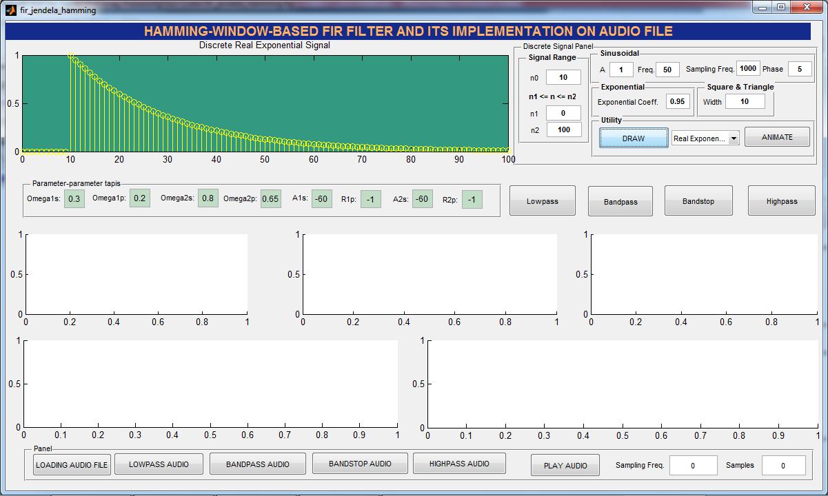
5. You can run the UI. Choose one of signals and then click DRAW button:


9. You can run the UI. Choose one of signals and then click DRAW button, choose one of window functions, and click on Lowpass button. The result is shown in figure below.


17. You can run the UI. Click LOAD AUDIO FILE button. The result is shown in figure below.


Here, you will build a desktop application (UI, user interface) to simulate how is filtered using FIR filter, Various Windows Based FIR Filter. A number of discrete signals are used as test signals are impulse, step, real exponential, sinusoidal, random, square, angled triangle, equilateral triangle, and trapezoidal signals. In the UI, this FIR filter is used to filter signals and audio file (wav) as well.
Follow these steps below:
1. Type this command on MATLAB prompt:
guide
The GUIDE Quick Start dialog box will show up, as shown in figure below:

2. Select the Blank GUI (Default) template, and then click OK:

3. Drag all components needed, as shown in figure below:

4. Right click on DRAW button and choose View Callbacks and then choose Callback. Define pbDraw_Callback() function below to read signals parameters and displays chosen signal in axes1 component:
% --- Executes on button press in pbDraw.
function pbDraw_Callback(hObject, eventdata, handles)
% hObject    handle to pbDraw (see GCBO)
% eventdata  reserved - to be defined in a future version of MATLAB
% handles    structure with handles and user data (see GUIDATA)
global n0;
global n1;
global x;

% Reads n0, n1, and n2
n0 = str2num(get(handles.n0,'String'));
n1 = str2num(get(handles.n1,'String'));
n2 = str2num(get(handles.n2,'String'));
exp = str2num(get(handles.expCoef,'String'));

% Reads parameters for sinusoidal
A = str2num(get(handles.A,'String'));
Freq = str2num(get(handles.Freq,'String'));
Fase = str2num(get(handles.Phase,'String'));
Fs = str2num(get(handles.Fs,'String'));

% Reads parameters for square and triangle signals
width = str2num(get(handles.width, 'String'));

% Choose option from popup menu popupmenusignal1
switch get(handles.popupmenusignal1,'Value')
    case 1
       n = [n1:n2]; x = [(n-n0) == 0];

       % Display discrete signal
       axes(handles.axes1)
       stem(n,x,'linewidth',2,'color','y');
       set(gca,'color',[0.4 0.6 0.5]);
       title('Discrete Impulse Signal');

    case 2
       n = [n1:n2]; x = [(n-n0) >= 0];
       % Display discrete signal
       axes(handles.axes1)
       stem(n,x,'linewidth',2,'color','y');
       set(gca,'color',[0.4 0.6 0.5]);
       title('Discrete Step Signal');

    case 3
       n = [n1:n2]; x = [(n-n0) >= 0].*[(exp).^(n-n0)];
       % Display discrete signal
       axes(handles.axes1)
       stem(n,x,'linewidth',1,'color','y');
       set(gca,'color',[0.4 0.6 0.5]);
       title('Discrete Real Exponential Signal');

    case 4
       n = [n1:n2]; x = [(n-n0) >= 0].*[A*sin(2*pi*(Freq)*((n-n0)/Fs)+Fase)];
       % Display discrete signal
       axes(handles.axes1)
       stem(n,x,'linewidth',2,'color','y');
       set(gca,'color',[0.4 0.6 0.5]);
       title('Discrete Sinusoidal Signal');

    case 5
       n = [n1:n2]; x = [(n-n0) >= 0].*(rand(1,(n2-n1+1))-0.5);
       % Display discrete signal
       axes(handles.axes1)
       stem(n,x,'linewidth',1,'color','y');
       set(gca,'color',[0.4 0.6 0.5]);
       title('Discrete Random Signal');

    case 6
       n = [n1:n2]; x = [(n-n0) >= 0];
       ny = [n1:n2]; xy = [(ny-width-n0-1) >= 0];
       x = x - xy;

       % Display discrete signal
       axes(handles.axes1)
       stem(n,x,'linewidth',1,'color','y');
       set(gca,'color',[0.4 0.6 0.5]);
       title('Discrete Square Signal');

    case 7
       n = [n1:n2]; x = n.*[n >= 0];
       ny = [n1:n2]; xy = ny.*[(ny-width-1) >= 0];
       x = (x - xy)/width;
       nb = [n1+n0:n2+n0];

       % Reads signal range
       set(handles.n1,'string',(n1+n0));
       set(handles.n2,'string',(n2+n0));

       % Display discrete signal
       axes(handles.axes1)
       stem(nb,x,'linewidth',1,'color','y');
       set(gca,'color',[0.4 0.6 0.5]);
       title('Discrete Angled Triangle Signal');

    case 8
       n = [n1:n2]; x = n.*[n >= 0];
       x2 = [zeros(1,width), x(1:end-width)];
       x1 = -x;
       x1 = [zeros(1,0.5*width), x1(1:end-0.5*width)];
       nb1 = n1+n0; nb2 = n2+n0;
       nb = [nb1:nb2];

       % Read signal range
       set(handles.n1,'string',(nb1));
       set(handles.n2,'string',(nb2));

       % Returns discrete equilateral triangle signal
       x = (x + 2*x1+x2)/(0.5*width);

       % Display discrete signal
       axes(handles.axes1)
       stem(nb,x,'linewidth',1,'color','y');
       set(gca,'color',[0.4 0.6 0.5]);
       title('Discrete Equilateral Triangle Signal');

    case 9
       n = [n1:n2]; x = n.*[n >= 0];
       x2 = [zeros(1,width), x(1:end-width)];
       x3 = [zeros(1,3*width), x(1:end-3*width)];
       x1 = x;
       x1 = [zeros(1,2*width), x1(1:end-2*width)];
       nb1 = n1+n0; nb2 = n2+n0;
       nb = [nb1:nb2];

       % Reads signal range
       set(handles.n1,'string',(nb1));
       set(handles.n2,'string',(nb2));

       % Returns discrete trapezoidal signal
       x = (x - x2 - x1 + x3)/width;

       % Display discrete signal
       axes(handles.axes1)
       stem(nb,x,'linewidth',1,'color','y');
       set(gca,'color',[0.4 0.6 0.5]);
       title('Discrete Trapezoidal Signal');
end
5. You can run the UI. Choose one of signals and then click DRAW button:

6. Set the String property of popupmenuwindow with Rectangular, Bartlett, Hann, Hamming, Blackman, and Kaiser.

7. Define ideal_lp() function (save to m file) to calculate ideal lowpass filter, given the cutoff frequency and filter length:
function hd = ideal_lp(wc,M)
% Calculates ideal lowpass filter
% -------------------------
% [hd]= lp_ideal(wc,M)
% wc = cutoff frequency in radian
% M = ideal filter length
%
alpha = (M-1)/2; n = [0:1:(M-1)];
m = n - alpha; fc = wc/pi; hd = fc*sinc(fc*m);
8. Right click on Lowpass button and choose View Callbacks and then choose Callback. Define pbLowpass_Callback() function below to read signals parameters and displays ideal lowpass impulse response, window function (based on window chosen from popupmenuwindow component), actual lowpass impulse response, lowpass magnitude response, and filtered signal:
% --- Executes on button press in pbLowpass.
function pbLowpass_Callback(hObject, eventdata, handles)
% hObject    handle to pbLowpass (see GCBO)
% eventdata  reserved - to be defined in a future version of MATLAB
% handles    structure with handles and user data (see GUIDATA)
global x;

% Reads all filter spesifications
As = str2num(get(handles.As,'String'));
ws = str2num(get(handles.omega_s,'String'));
Rp = str2num(get(handles.Rp,'String'));
wp = str2num(get(handles.omega_p,'String'));

ws=ws*pi; wp=wp*pi;
bandwidth = ws - wp;
M = ceil(6.6*pi/bandwidth) + 1;
n=[0:1:M-1];
wc = (ws+wp)/2; % cutoff frequency of LPF

% Choosing option from popup menu
switch get(handles.popupmenuwindow,'Value')
    case 1
        j=boxcar(M);
    case 2
        j=bartlett(M);
    case 3
        j=hann(M);
    case 4
        j=hamming(M);
    case 5
        j=blackman(M);
    case 6
        beta = 0.1102*(As-8.7);
        j=kaiser(M,beta);
end

hd = ideal_lp(wc,M); h = hd' .* j;
[db,mag,pha,grd,w] = freqz_m(h,[1]); delta_w = 2*pi/1000;

% Actual ripple passband
Rp = -(min(db(1:1:wp/delta_w+1)));

% Minimal stopband attenuation
As = -round(max(db(ws/delta_w+1:1:501)));

axes(handles.axes7);
stem(n,hd, 'color','w'); title('Ideal Lowpass Impulse Response')
set(gca,'color',[0.6,0.2,0.1]);
axis([0 M-1 min(hd) max(hd)]); xlabel('n'); ylabel('hd(n)')

axes(handles.axes8);
stem(n,j,'color','w');title('Window Function')
axis([0 M-1 0 1.1]); xlabel('n'); ylabel('w(n)')
set(gca,'color',[0.6,0.2,0.1]);

axes(handles.axes9);
stem(n,h,'color','w');title('Actual Lowpass Impulse')
axis([0 M-1 min(h) max(h)]); xlabel('n'); ylabel('h(n)')
set(gca,'color',[0.6,0.2,0.1]);

axes(handles.axes3);
plot(w/pi,db, 'linewidth',2,'color','y');
title('Magnitude Response in dB');grid
axis([0 1 min(db) max(db)]);
xlabel('Frequency in pi unit'); ylabel('dB')
set(gca,'color',[0.6,0.2,0.1]);

% Calculates filtered signal
y = conv(double(x),double(h), 'same');

axes(handles.axes2);
t = 0:length(y)-1;
stem(t,y,'linewidth',1,'color','g');
title('Filtered Signal')
set(gca,'color',[0.6,0.2,0.1]);
9. You can run the UI. Choose one of signals and then click DRAW button, choose one of window functions, and click on Lowpass button. The result is shown in figure below.

10. Right click on Highpass button and choose View Callbacks and then choose Callback. Define pbHighpass_Callback() function below to read signals parameters and displays ideal highpass impulse response, window function (based on window chosen from popupmenuwindow component), actual highpass impulse response, highpass magnitude response, and filtered signal:
% --- Executes on button press in pbHighpass.
function pbHighpass_Callback(hObject, eventdata, handles)
% hObject    handle to pbHighpass (see GCBO)
% eventdata  reserved - to be defined in a future version of MATLAB
% handles    structure with handles and user data (see GUIDATA)

global x;

% Reads all filter spesifications
As = str2num(get(handles.As,'String'));
ws = str2num(get(handles.omega_s,'String'));
Rp = str2num(get(handles.Rp,'String'));
wp = str2num(get(handles.omega_p,'String'));

ws=ws*pi; wp=wp*pi;
bandwidth = ws - wp;
M = ceil(6.6*pi/bandwidth) + 1;
n=[0:1:M-1];
wc = (ws+wp)/2; % cutoff frequency of HPF

% Choosing option from popup menu
switch get(handles.popupmenuwindow,'Value')
    case 1
        j=boxcar(M);
    case 2
        j=bartlett(M);
    case 3
        j=hann(M);
    case 4
        j=hamming(M);
    case 5
        j=blackman(M);
    case 6
        beta = 0.1102*(As-8.7);
        j=kaiser(M,beta);
end

hd = ideal_lp(pi,M) - ideal_lp(wc,M);
h = hd' .* j;
[db,mag,pha,grd,w] = freqz_m(h,[1]); delta_w = 2*pi/1000;

% Actual ripple passband
Rp = -(min(db(1:1:wp/delta_w+1)));

% Minimal stopband attenuation
As = -round(max(db(ws/delta_w+1:1:501)));

axes(handles.axes7);
stem(n,hd, 'color','w'); title('Ideal Highpass Impulse Response')
set(gca,'color',[0.6,0.2,0.1]);
axis([0 M-1 min(hd) max(hd)]); xlabel('n'); ylabel('hd(n)')

axes(handles.axes8);
stem(n,j,'color','w');title('Window Function')
axis([0 M-1 0 1.1]); xlabel('n'); ylabel('w(n)')
set(gca,'color',[0.6,0.2,0.1]);

axes(handles.axes9);
stem(n,h,'color','w');title('Actual Highpass Impulse')
axis([0 M-1 min(h) max(h)]); xlabel('n'); ylabel('h(n)')
set(gca,'color',[0.6,0.2,0.1]);

axes(handles.axes3);
plot(w/pi,db, 'linewidth',2,'color','y');
title('Magnitude Response in dB');grid
axis([0 1 min(db) max(db)]);
xlabel('Frequency in pi unit'); ylabel('dB')
set(gca,'color',[0.6,0.2,0.1]);

% Calculates filtered signal
y = conv(double(x),double(h), 'same');

axes(handles.axes2);
t = 0:length(y)-1;
stem(t,y,'linewidth',1,'color','g');
title('Filtered Signal')
set(gca,'color',[0.6,0.2,0.1]);
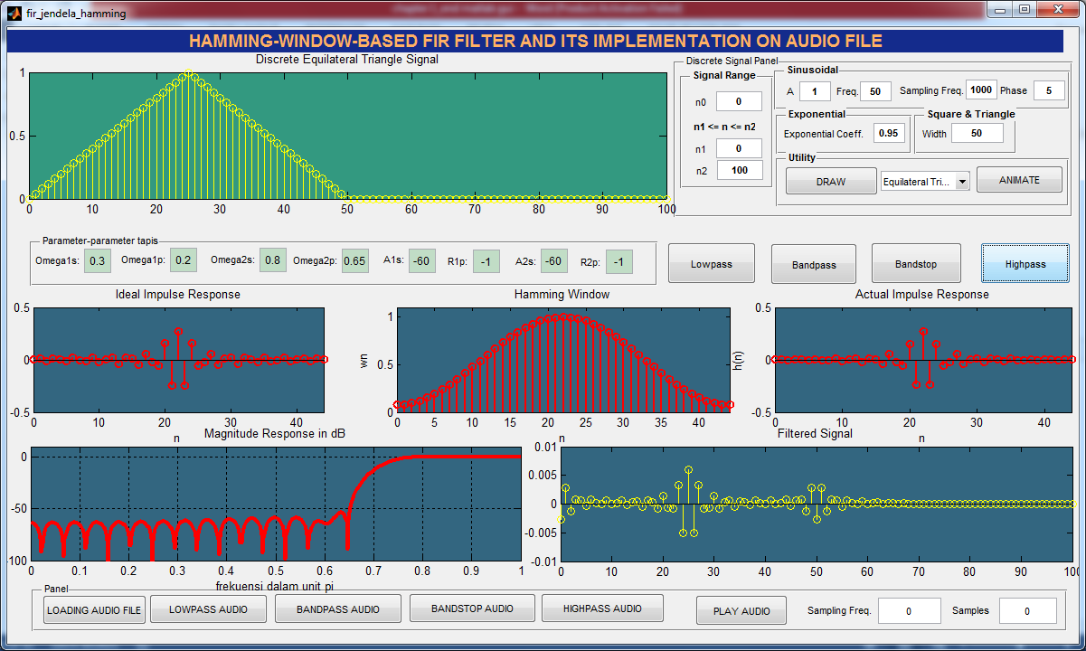
11. You can run the UI. Choose one of signals and then click DRAW button, choose one of window functions, and click on Highpass button. The result is shown in figure below.

12. Right click on Bandpass button and choose View Callbacks and then choose Callback. Define pbBandpass_Callback() function below to read signals parameters and displays ideal bandpass impulse response, window function (based on window chosen from popupmenuwindow component), actual bandpass impulse response, bandpass magnitude response, and filtered signal:
% --- Executes on button press in pbBandpass.
function pbBandpass_Callback(hObject, eventdata, handles)
% hObject    handle to pbBandpass (see GCBO)
% eventdata  reserved - to be defined in a future version of MATLAB
% handles    structure with handles and user data (see GUIDATA)

global x;

% Reads all filter spesifications
As = str2num(get(handles.As,'String'));
ws = str2num(get(handles.omega_s,'String'));
Rp = str2num(get(handles.Rp,'String'));
wp = str2num(get(handles.omega_p,'String'));
wp2 = str2num(get(handles.wp2,'String'));
ws2 = str2num(get(handles.ws2,'String'));

ws=ws*pi; wp=wp*pi; wp2=wp2*pi; ws2=ws2*pi;
bandwidth = min((ws-wp),(ws2-wp2)); M = ceil(11*pi/bandwidth) + 1;
n=[0:1:M-1]; wc1 = (ws+wp)/2;
wc2 = (wp2+ws2)/2;

% Choosing option from popup menu
switch get(handles.popupmenuwindow,'Value')
    case 1
        j=boxcar(M);
    case 2
        j=bartlett(M);
    case 3
        j=hann(M);
    case 4
        j=hamming(M);
    case 5
        j=blackman(M);
    case 6
        beta = 0.1102*(As-8.7);
        j=kaiser(M,beta);
end

% Bandpass
hd = ideal_lp(wc2,M) - ideal_lp(wc1,M);
h = hd' .* j;
[db,mag,pha,grd,w] = freqz_m(h,[1]); delta_w = 2*pi/1000;

% Actual ripple passband
Rp = -(min(db(1:1:wp/delta_w+1)));

% Minimal stopband attenuation
As = -round(max(db(ws/delta_w+1:1:501)));

axes(handles.axes7);
stem(n,hd, 'color','w'); title('Ideal Bandpass Impulse Response')
set(gca,'color',[0.6,0.2,0.1]);
axis([0 M-1 min(hd) max(hd)]); xlabel('n'); ylabel('hd(n)')

axes(handles.axes8);
stem(n,j,'color','w');title('Window Function')
axis([0 M-1 0 1.1]); xlabel('n'); ylabel('w(n)')
set(gca,'color',[0.6,0.2,0.1]);

axes(handles.axes9);
stem(n,h,'color','w');title('Actual Bandpass Impulse')
axis([0 M-1 min(h) max(h)]); xlabel('n'); ylabel('h(n)')
set(gca,'color',[0.6,0.2,0.1]);

axes(handles.axes3);
plot(w/pi,db, 'linewidth',2,'color','y');
title('Magnitude Response in dB');grid
axis([0 1 min(db) max(db)]);
xlabel('Frequency in pi unit'); ylabel('dB')
set(gca,'color',[0.6,0.2,0.1]);

% Calculates filtered signal
y = conv(double(x),double(h), 'same');

axes(handles.axes2);
t = 0:length(y)-1;
stem(t,y,'linewidth',1,'color','g');
title('Filtered Signal')
set(gca,'color',[0.6,0.2,0.1]);
13. You can run the UI. Choose one of signals and then click DRAW button, choose one of window functions, and click on Bandpass button. The result is shown in figure below.

14. Right click on Bandstop button and choose View Callbacks and then choose Callback. Define pbBandstop_Callback() function below to read signals parameters and displays ideal bandstop impulse response, window function (based on window chosen from popupmenuwindow component), actual bandstop impulse response, bandstop magnitude response, and filtered signal:
% --- Executes on button press in pbBandpass.
function pbBandpass_Callback(hObject, eventdata, handles)
% hObject    handle to pbBandpass (see GCBO)
% eventdata  reserved - to be defined in a future version of MATLAB
% handles    structure with handles and user data (see GUIDATA)
% --- Executes on button press in pbBandstop.
function pbBandstop_Callback(hObject, eventdata, handles)
% hObject    handle to pbBandstop (see GCBO)
% eventdata  reserved - to be defined in a future version of MATLAB
% handles    structure with handles and user data (see GUIDATA)

global x;

% Reads all filter spesifications
As = str2num(get(handles.As,'String'));
ws = str2num(get(handles.omega_s,'String'));
Rp = str2num(get(handles.Rp,'String'));
wp = str2num(get(handles.omega_p,'String'));
wp2 = str2num(get(handles.wp2,'String'));
ws2 = str2num(get(handles.ws2,'String'));

ws=ws*pi; wp=wp*pi; wp2=wp2*pi; ws2=ws2*pi;
As = 60;
tr_width = min((ws-wp),(ws2-wp2)); M = ceil(11*pi/tr_width) + 1;

n=[0:1:M-1]; wc1 = (ws+wp)/2; wc2 = (wp2+ws2)/2;

% Choosing option from popup menu
switch get(handles.popupmenuwindow,'Value')
    case 1
        j=boxcar(M);
    case 2
        j=bartlett(M);
    case 3
        j=hann(M);
    case 4
        j=hamming(M);
    case 5
        j=blackman(M);
    case 6
        beta = 0.1102*(As-8.7);
        j=kaiser(M,beta);
end

% Bandstop
hd = ideal_lp(wc1,M) + ideal_lp(pi,M) - ideal_lp(wc2,M);
h = hd' .* j;
[db,mag,pha,grd,w] = freqz_m(h,[1]); delta_w = 2*pi/1000;

% Actual ripple passband
Rp = -(min(db(1:1:wp/delta_w+1)));

% Minimal stopband attenuation
As = -round(max(db(ws/delta_w+1:1:501)));

axes(handles.axes7);
stem(n,hd, 'color','w'); title('Ideal Bandstop Impulse Response')
set(gca,'color',[0.6,0.2,0.1]);
axis([0 M-1 min(hd) max(hd)]); xlabel('n'); ylabel('hd(n)')

axes(handles.axes8);
stem(n,j,'color','w');title('Window Function')
axis([0 M-1 0 1.1]); xlabel('n'); ylabel('w(n)')
set(gca,'color',[0.6,0.2,0.1]);

axes(handles.axes9);
stem(n,h,'color','w');title('Actual Bandstop Impulse')
axis([0 M-1 min(h) max(h)]); xlabel('n'); ylabel('h(n)')
set(gca,'color',[0.6,0.2,0.1]);

axes(handles.axes3);
plot(w/pi,db, 'linewidth',2,'color','y');
title('Magnitude Response in dB');grid
axis([0 1 min(db) max(db)]);
xlabel('Frequency in pi unit'); ylabel('dB')
set(gca,'color',[0.6,0.2,0.1]);

% Calculates filtered signal
y = conv(double(x),double(h), 'same');

axes(handles.axes2);
t = 0:length(y)-1;
stem(t,y,'linewidth',1,'color','g');
title('Filtered Signal')
set(gca,'color',[0.6,0.2,0.1]);
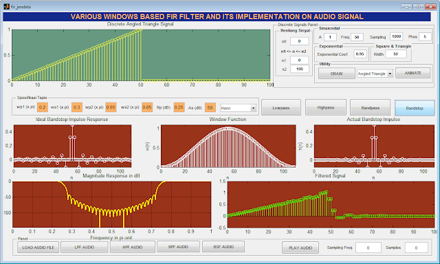
15. You can run the UI. Choose one of signals and then click DRAW button, choose one of window functions, and click on Bandstop button. The result is shown in figure below.

16. Right click on LOAD AUDIO FILE button and choose View Callbacks and then choose Callback. Define pbLoadAudioFile_Callback() function below to read audio file and display its spectrum:
% --- Executes on button press in pbLoadAudioFile.
function pbLoadAudioFile_Callback(hObject, eventdata, handles)
% hObject    handle to pbLoadAudioFile (see GCBO)
% eventdata  reserved - to be defined in a future version of MATLAB
% handles    structure with handles and user data (see GUIDATA)

global x_audio;

[filename,path] = uigetfile({'*.wav'},'Muat File Wav');
[x,Fs] = audioread([path '/' filename]);
handles.x = x ./ max(abs(x));
handles.Fs = Fs;

axes(handles.axes2);
waktu = 0:1/Fs:(length(handles.x)-1)/Fs;
plot(waktu, handles.x,'linewidth',1,'color','r');
set(gca,'color',[0.1,0.2,0.8]);
axis([0 max(waktu) -1 1]); title('Audio Signal');

axes(handles.axes3);
specgram(handles.x, 1024, handles.Fs);
set(gca,'color',[0.2,0.2,0.8]);
title('Signal Spectrum');
handles.fileLoad = 1;

handles.fileNoise = 0;
handles.fileFinal = 0;

set(handles.SamplingFreq, 'String', num2str(Fs));
set(handles.NSamples, 'String', num2str(length(handles.x)));

x_audio = handles.x;
guidata(hObject, handles);
17. You can run the UI. Click LOAD AUDIO FILE button. The result is shown in figure below.

18. Right click on LPF AUDIO button and choose View Callbacks and then choose Callback. Define pbLPFAudio_Callback() function below to calculate and display filtered signal and its spectrum:
% --- Executes on button press in pbLPFAudio.
function pbLPFAudio_Callback(hObject, eventdata, handles)
% hObject    handle to pbLPFAudio (see GCBO)
% eventdata  reserved - to be defined in a future version of MATLAB
% handles    structure with handles and user data (see GUIDATA)

global x;
global x_audio;

% Reads all filter spesification
As = str2num(get(handles.As,'String'));
ws = str2num(get(handles.omega_s,'String'));
Rp = str2num(get(handles.Rp,'String'));
wp = str2num(get(handles.omega_p,'String'));

ws=ws*pi; wp=wp*pi;
tr_width = ws - wp;
M = ceil(6.6*pi/tr_width) + 1;
n=[0:1:M-1];
wc = (ws+wp)/2;

% Choose window function
switch get(handles.popupmenuwindow,'Value')
    case 1
        j=boxcar(M);
    case 2
        j=bartlett(M);
    case 3
        j=hann(M);
    case 4
        j=hamming(M);
    case 5
        j=blackman(M);
    case 6
        beta = 0.1102*(As-8.7);
        j=kaiser(M,beta);
end

hd = ideal_lp(wc,M); h = hd' .* j;

% Calculates filtered signal
y = conv(hd,x_audio);

axes(handles.axes2);
t = 0:length(y)-1;
plot(t,y,'linewidth',1,'color','r');
title('Filtered Signal')
set(gca,'color',[0.1,0.2,0.8]);

axes(handles.axes3)
specgram(y, 1024, handles.Fs);
title('Signal Spectrum');
handles.fileLoad = 1;
set(gca,'color',[0.1,0.2,0.8]);
handles.x=y;
guidata(hObject, handles);
19. You can run the UI. Click LOAD AUDIO FILE button and then click LPF Audio button. The result is shown in figure below.

20. Right click on HPF AUDIO button and choose View Callbacks and then choose Callback. Define pbHPFAudio_Callback() function below to calculate and display filtered signal and its spectrum:
% --- Executes on button press in pbHPFAudio.
function pbHPFAudio_Callback(hObject, eventdata, handles)
% hObject    handle to pbHPFAudio (see GCBO)
% eventdata  reserved - to be defined in a future version of MATLAB
% handles    structure with handles and user data (see GUIDATA)

global x;
global x_audio;

% Reads all filter spesification
As = str2num(get(handles.As,'String'));
ws = str2num(get(handles.omega_s,'String'));
Rp = str2num(get(handles.Rp,'String'));
wp = str2num(get(handles.omega_p,'String'));

% Calculates cutoff frequency
bandwidth = ws - wp;
M = ceil(6.6*pi/bandwidth) + 1;
n=[0:1:M-1];
wc = (ws+wp)/2;

% Choose window function
switch get(handles.popupmenuwindow,'Value')
    case 1
        j=boxcar(M);
    case 2
        j=bartlett(M);
    case 3
        j=hann(M);
    case 4
        j=hamming(M);
    case 5
        j=blackman(M);
    case 6
        beta = 0.1102*(As-8.7);
        j=kaiser(M,beta);
end

% HPF
hd = ideal_lp(pi,M) - ideal_lp(wc,M);
h = hd' .* j;

% Calculates filtered signal
y = conv(h,x_audio);

axes(handles.axes2);
t = 0:length(y)-1;
plot(t,y,'linewidth',1,'color','r');title('Filtered Signal')
set(gca,'color', [0.1,0.2,0.8]);

axes(handles.axes3)
specgram(y, 1024, handles.Fs);
title('Spektrum Sinyal');
handles.fileLoad = 1;
set(gca,'color', [0.1,0.2,0.8]);
handles.x=y;
guidata(hObject, handles);
21. You can run the UI. Click LOAD AUDIO FILE button and then click HPF Audio button. The result is shown in figure below.