This content is powered by Balige Publishing. Visit this link (collaboration with Rismon Hasiholan Sianipar) PART 1 PART 2
In this tutorial, you will learn how to use Pandas, NumPy, Scikit-Learn, and other libraries to perform simple classification using perceptron and Adaline (adaptive linear neuron). The dataset used is Iris dataset directly from the UCI Machine Learning Repository.
Tutorial Steps To Implement Perceptron Using Scikit-Learn with PyQt
Step 1: Open gui_perceptron.ui form with Qt Designer from Chapter 1 and save it as gui_scikit.ui.

Step 3: Write this script and save it as Scikit_Classifier.py:
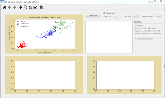
Step 4: Run Scikit_Classifier.py and the result is shown in Figure below.

Step 5: Define load_data() and display_data() functions to display data as follows:
Step 6: Connect clicked() signal of pbLoad widget with load_data() function and put it inside __init__() method:
Step 7: Run Scikit_Classifier.py to the result as shown in Figure below.
Step 8: Define display_table() and write_df_to_qtable() functions to display the data on table as follows:
Step 9: Invoke display_table() function from display_data() as follows:
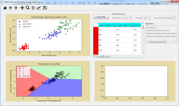
Step 10: Run Scikit_Classifier.py, click Load Data button, and you will see the data presented in tableData widget as shown in Figure below.

Step 11: Define display_decision() function to display decision regions for the three features using perceptron classifier as follows:
Step 12: Define algo_NN() and invoke display_decision() function from it. The algo_NN() also split the dataset into separate training and test datasets, standardize the features using the StandardScaler, and train the perceptron:
Step 13: Invoke algo_NN() function from display_data() function:
Step 14: Run Scikit_Classifier.py to see the decision regions as shown in Figure below.
Step 15: Enable gbNNParam widget and disable pbLoad widget after user clicks Load Data button as follows:
Step 16: Read the value property of sbIter, dsbRatio, and dsbRate, and put them inside algo_NN() function.
Assign the value of sbIter to test_size input parameter in train_test_split() function and assign the value of dsbRatio and dsbRate to initialize Perceptron object as follows:
Step 17: Connect valueChanged() signal of sbIter, dsbRate, and dsbRatio widget to algo_NN() function as follows:
Step 18: Run Scikit_Classifier.py to see the decision regions. You now can change the value of data ratio, the maximum number of iteration, and learning rate as shown in both Figures below.


Step 19: Now, you wil draw graph bar on widgetEpoch. The graph will consist of some accuracies of data ratio versus learning rate.
Step 20: Define graph() function to draw graph bar on widgetEpoch as follows:
Step 21: Invoke graph() from algo_NN() function:
Step 22: Run Scikit_Classifier.py and click Load Data button to see the graph as shown in Figure below.
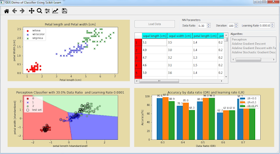
Change data ratio to 0.6 and you can see the result as shown in Figure below.

Then change learning rate to 0.1 and you can see the result as shown in Figure below.

Below is the full script of Scikit_Classifier.py so far:
Learn From Scratch Neural Networks Using PyQt: Part 4
In this tutorial, you will learn how to use Pandas, NumPy, Scikit-Learn, and other libraries to perform simple classification using perceptron and Adaline (adaptive linear neuron). The dataset used is Iris dataset directly from the UCI Machine Learning Repository.
Tutorial Steps To Implement Perceptron Using Scikit-Learn with PyQt
Step 1: Open gui_perceptron.ui form with Qt Designer from Chapter 1 and save it as gui_scikit.ui.
Step 2: Delete sbLength widget and add into new form a Double Spin Box widget. Set its objectName property as dsbRatio. Set its minimum, maximum, singleStep, and value properties to 0.1, 1, 0.1, and 0.3.
Add a Label widget and place it next to the new double spin box widget. Set its text property to Data Ratio.
The new form looks as shown in Figure below.

Step 3: Write this script and save it as Scikit_Classifier.py:
#Scikit_Classifier.py
from PyQt5.QtWidgets import *
from PyQt5.uic import loadUi
from matplotlib.backends.backend_qt5agg import (NavigationToolbar2QT as NavigationToolbar)
from matplotlib.colors import ListedColormap
from sklearn import datasets
from sklearn.preprocessing import StandardScaler
from sklearn.model_selection import train_test_split
from sklearn.linear_model import Perceptron
from sklearn.metrics import accuracy_score
import numpy as np
import pandas as pd

class DemoGUIScikit(QMainWindow):
    def __init__(self):
        QMainWindow.__init__(self)
        loadUi("gui_scikit.ui",self)

        self.setWindowTitle("GUI Demo of Classifier Using Scikit-Learn")
        self.addToolBar(NavigationToolbar(self.widgetData.canvas, self))
        self.gbNNParam.setEnabled(False)
        self.listAlgorithm.setEnabled(False)

if __name__ == '__main__':
    import sys
    app = QApplication(sys.argv)
    ex = DemoGUIScikit()
    ex.show()
    sys.exit(app.exec_())
Step 4: Run Scikit_Classifier.py and the result is shown in Figure below.

Step 5: Define load_data() and display_data() functions to display data as follows:
def load_data(self):
    #Load data into matrix X and vector y
    iris = datasets.load_iris()
    self.X = iris.data[:, [2, 3]]
    self.y = iris.target
    self.display_data(self.X, self.widgetData.canvas)

def display_data(self,X,axisWidget):
    # plot data
    axisWidget.axis1.clear()
    axisWidget.axis1.scatter(X[:50, 0], X[:50, 1],
        color='red', marker='o', label='setosa')

    axisWidget.axis1.scatter(X[50:100, 0], X[50:100, 1],
        color='blue', marker='x', label='versicolor')

    axisWidget.axis1.scatter(X[100:150, 0], X[100:150, 1],
        color='green', marker='x', label='virginica')

    axisWidget.axis1.set_xlabel('Petal length [cm]')
    axisWidget.axis1.set_ylabel('petal Width [cm]')
    axisWidget.axis1.legend(loc='upper left')

    title = 'Petal length and Petal width [cm]'
    axisWidget.axis1.set_title(title)
    axisWidget.draw()
Step 6: Connect clicked() signal of pbLoad widget with load_data() function and put it inside __init__() method:
self.pbLoad.clicked.connect(self.load_data)
Step 7: Run Scikit_Classifier.py to the result as shown in Figure below.

Step 8: Define display_table() and write_df_to_qtable() functions to display the data on table as follows:
def display_table(self):
    data = datasets.load_iris()
    df = pd.DataFrame(np.column_stack(\
            (data.data, data.target)), \
            columns = data.feature_names+['target'])
    df['label'] = \
            df.target.replace(dict(enumerate(data.target_names)))

    # show data on table widget
    self.write_df_to_qtable(df,self.tableData)
    self.tableData.setHorizontalHeaderLabels(data.feature_names)

    styleH = "::section {""background-color: cyan; }"
    self.tableData.horizontalHeader().setStyleSheet(styleH)

    styleV = "::section {""background-color: red; }"
    self.tableData.verticalHeader().setStyleSheet(styleV)

# Takes a df and writes it to a qtable provided. df headers
# become qtable headers
@staticmethod
def write_df_to_qtable(df,table):
    table.setRowCount(df.shape[0])
    table.setColumnCount(df.shape[1])

    # getting data from df is computationally costly
    # so convert it to array first
    df_array = df.values
    for row in range(df.shape[0]):
        for col in range(df.shape[1]):
            table.setItem(row, col, \
                QTableWidgetItem(str(df_array[row,col])))
Step 9: Invoke display_table() function from display_data() as follows:
def display_data(self,X,axisWidget):
    # plot data
    axisWidget.axis1.clear()
    axisWidget.axis1.scatter(X[:50, 0], X[:50, 1],
        color='red', marker='o', label='setosa')

    axisWidget.axis1.scatter(X[50:100, 0], X[50:100, 1],
        color='blue', marker='x', label='versicolor')

    axisWidget.axis1.scatter(X[100:150, 0], X[100:150, 1],
        color='green', marker='x', label='virginica')

    axisWidget.axis1.set_xlabel('Petal length [cm]')
    axisWidget.axis1.set_ylabel('petal Width [cm]')
    axisWidget.axis1.legend(loc='upper left')

    title = 'Petal length and Petal width [cm]'
    axisWidget.axis1.set_title(title)
    axisWidget.draw()

    #displays data on table widget
    self.display_table()
Step 10: Run Scikit_Classifier.py, click Load Data button, and you will see the data presented in tableData widget as shown in Figure below.

Step 11: Define display_decision() function to display decision regions for the three features using perceptron classifier as follows:
def display_decision(self, X, y, classifier, axisWidget, title, test_idx=None, resolution=0.01):
    # setup marker generator and color map
    markers = ('s', 'x', 'o', '^', 'v')
    colors = ('red', 'blue', 'lightgreen', 'gray', 'cyan')
    cmap = ListedColormap(colors[:len(np.unique(y))])

    # plot the decision surface
    x1_min, x1_max = X[:, 0].min() - 1, X[:, 0].max() + 1
    x2_min, x2_max = X[:, 1].min() - 1, X[:, 1].max() + 1
    xx1, xx2 = np.meshgrid(np.arange(x1_min, x1_max, resolution),\
        np.arange(x2_min, x2_max, resolution))

    Z = classifier.predict(np.array([xx1.ravel(), xx2.ravel()]).T)
    Z = Z.reshape(xx1.shape)

    axisWidget.axis1.clear()
    axisWidget.axis1.contourf(xx1, xx2, Z, alpha=0.5, cmap=cmap)
    axisWidget.axis1.set_xlim(xx1.min(), xx1.max())
    axisWidget.axis1.set_ylim(xx2.min(), xx2.max())

    for idx, cl in enumerate(np.unique(y)):
        axisWidget.axis1.scatter(x=X[y == cl, 0], y=X[y == cl, 1],
                    alpha=0.8, c=colors[idx],
                    marker=markers[idx], label=cl,
                    edgecolor='black')

    # highlight test samples
    if test_idx:
        # plot all samples
        X_test, y_test = X[test_idx, :], y[test_idx]
        axisWidget.axis1.scatter(X_test[:, 0], X_test[:, 1],
                    c='', edgecolor='black', alpha=1.0,
                    linewidth=1, marker='o',
                    s=100, label='test set')

    axisWidget.axis1.set_xlabel('petal length [standardized]')
    axisWidget.axis1.set_ylabel('petal width [standardized]')
    axisWidget.axis1.set_label('petal width [standardized]')
    axisWidget.axis1.legend(loc='upper left')
    axisWidget.axis1.set_title(title)
    axisWidget.draw()
Step 12: Define algo_NN() and invoke display_decision() function from it. The algo_NN() also split the dataset into separate training and test datasets, standardize the features using the StandardScaler, and train the perceptron:
def algo_NN(self):
    #Splits the dataset into separate training and test datasets
    X_train, X_test, y_train, y_test = train_test_split(self.X, \
        self.y, test_size=0.3, random_state=1, stratify=self.y)

    #standardizes the features using the StandardScaler
    sc = StandardScaler()
    sc.fit(X_train)
    X_train_std = sc.transform(X_train)
    X_test_std = sc.transform(X_test)

    #Trains perceptron
    ppn = Perceptron(max_iter=100, eta0=0.1, random_state=1)
    ppn.fit(X_train_std, y_train)

    X_combined_std = np.vstack((X_train_std, X_test_std))
    y_combined = np.hstack((y_train, y_test))

    strTitle = 'Perceptron Classifier'
    self.display_decision(X=X_combined_std, y=y_combined, \
        classifier=ppn, axisWidget=self.widgetDecision.canvas, \
        title=strTitle, test_idx=range(105, 150))
Step 13: Invoke algo_NN() function from display_data() function:
def display_data(self,X,axisWidget):
    # plot data
    axisWidget.axis1.clear()
    axisWidget.axis1.scatter(X[:50, 0], X[:50, 1],
        color='red', marker='o', label='setosa')

    axisWidget.axis1.scatter(X[50:100, 0], X[50:100, 1],
        color='blue', marker='x', label='versicolor')

    axisWidget.axis1.scatter(X[100:150, 0], X[100:150, 1],
        color='green', marker='x', label='virginica')

    axisWidget.axis1.set_xlabel('Petal length [cm]')
    axisWidget.axis1.set_ylabel('petal Width [cm]')
    axisWidget.axis1.legend(loc='upper left')

    title = 'Petal length and Petal width [cm]'
    axisWidget.axis1.set_title(title)
    axisWidget.draw()

    #displays data on table widget
    self.display_table()

    #Displays decision regions
    self.algo_NN()
Step 14: Run Scikit_Classifier.py to see the decision regions as shown in Figure below.

Step 15: Enable gbNNParam widget and disable pbLoad widget after user clicks Load Data button as follows:
def load_data(self):
    #Load data into matrix X and vector y
    iris = datasets.load_iris()
    self.X = iris.data[:, [2, 3]]
    self.y = iris.target
    self.display_data(self.X, self.widgetData.canvas)
    self.gbNNParam.setEnabled(True)
    self.pbLoad.setEnabled(False)
Step 16: Read the value property of sbIter, dsbRatio, and dsbRate, and put them inside algo_NN() function.
Assign the value of sbIter to test_size input parameter in train_test_split() function and assign the value of dsbRatio and dsbRate to initialize Perceptron object as follows:
def algo_NN(self):
    iterNum = self.sbIter.value()
    ratio = self.dsbRatio.value()
    self.dsbRate.setDecimals(5)
    learningRate = self.dsbRate.value()

    #Splits the dataset into separate training and test datasets
    X_train, X_test, y_train, y_test = train_test_split(self.X, \
        self.y, test_size=ratio, random_state=1, stratify=self.y)

    #standardizes the features using the StandardScaler
    sc = StandardScaler()
    sc.fit(X_train)
    X_train_std = sc.transform(X_train)
    X_test_std = sc.transform(X_test)

    #Trains perceptron
    ppn = Perceptron(max_iter=iterNum, eta0=learningRate, \
        random_state=1)
    ppn.fit(X_train_std, y_train)

    X_combined_std = np.vstack((X_train_std, X_test_std))
    y_combined = np.hstack((y_train, y_test))

    strTitle = 'Perceptron Classifier with ' + \
        str(ratio*100) + '% Data Ratio '
        strTitle += ' and Learning Rate ' +str(learningRate)

    self.display_decision(X=X_combined_std, y=y_combined, \
        classifier=ppn, axisWidget=self.widgetDecision.canvas, \
        title=strTitle, test_idx=range(105, 150))
Step 17: Connect valueChanged() signal of sbIter, dsbRate, and dsbRatio widget to algo_NN() function as follows:
def __init__(self):
    QMainWindow.__init__(self)
    loadUi("gui_scikit.ui",self)

    self.setWindowTitle("GUI Demo of Classifier Using Scikit-Learn")
    self.addToolBar(NavigationToolbar(self.widgetData.canvas, self))
    self.gbNNParam.setEnabled(False)
    self.listAlgorithm.setEnabled(False)

    self.pbLoad.clicked.connect(self.load_data)
    self.sbIter.valueChanged.connect(self.algo_NN)
    self.dsbRate.valueChanged.connect(self.algo_NN)
    self.dsbRatio.valueChanged.connect(self.algo_NN)
Step 18: Run Scikit_Classifier.py to see the decision regions. You now can change the value of data ratio, the maximum number of iteration, and learning rate as shown in both Figures below.


Step 19: Now, you wil draw graph bar on widgetEpoch. The graph will consist of some accuracies of data ratio versus learning rate.
Define accuracy_perceptron() function to calculate percepton prediction accuracy for certain data ratio and learning rate as follows:
def accuracy_perceptron(self, ratio,learningRate):
    #Splits the dataset into separate training and test datasets
    X_train, X_test, y_train, y_test = train_test_split(self.X, \
        self.y, test_size=ratio, random_state=1, stratify=self.y)

    #standardizes the features using the StandardScaler
    sc = StandardScaler()
    sc.fit(X_train)
    X_train_std = sc.transform(X_train)
    X_test_std = sc.transform(X_test)

    #Trains perceptron
    ppn = Perceptron(max_iter=100, eta0=learningRate, random_state=1)
    ppn.fit(X_train_std, y_train)

    #Makes prediction
    y_pred = ppn.predict(X_test_std)

    #Calculates classification accuracy (in percent)
    acc = round(100*accuracy_score(y_test, y_pred),1)
    return acc
Step 20: Define graph() function to draw graph bar on widgetEpoch as follows:
def graph(self,axisWidget,func):
    ratio = self.dsbRatio.value()
    learningRate = self.dsbRate.value()

    if (ratio+0.4) < 1 :
        rangeDR = [ratio,ratio+0.1,ratio+0.2,ratio+0.3,ratio+0.4]
    else :
       rangeDR = [ratio-0.4,ratio-0.3,ratio-0.2,ratio-0.1,ratio]

    labels = [str(round(rangeDR[0],2)), str(round(rangeDR[1],2)), \
              str(round(rangeDR[2],2)), str(round(rangeDR[3],2)), \
              str(round(rangeDR[4],2))]

    LR01 = []
    for i in rangeDR:
        acc = func(i,learningRate)
        LR01.append(acc)

    LR001 = []
    for i in rangeDR:
        acc = func(i,learningRate+0.1)
        LR001.append(acc)

    LR0001 = []
    for i in rangeDR:
        acc = func(i,learningRate+0.25)
        LR0001.append(acc)

    x = np.arange(len(labels))  # the label locations
    width = 0.3  # the width of the bars

    strLabel1 = 'LR=' + str(round(learningRate, 2))
    strLabel2 = 'LR=' + str(round(learningRate+0.1, 2))
    strLabel3 = 'LR=' + str(round(learningRate+0.25, 2))
    axisWidget.axis1.clear()
    rects1 = axisWidget.axis1.bar(x - width/2, LR01, \
        width, label=strLabel1)
    rects2 = axisWidget.axis1.bar(x + width/2, LR001, \
        width, label=strLabel2)
    rects3 = axisWidget.axis1.bar(x + 3*width/2, LR0001, \
        width, label=strLabel3)

    # Add some text for labels, title and custom x-axis tick labels, etc.
    axisWidget.axis1.set_ylabel('Accuracy(%)')
    axisWidget.axis1.set_xlabel('Data Ratio (DR)')
    axisWidget.axis1.set_title(\
        'Accuracy by data ratio (DR) and learning rate (LR)')
    axisWidget.axis1.set_xticks(x)
    axisWidget.axis1.set_xticklabels(labels)
    axisWidget.axis1.legend()
    #axisWidget.axis1.set_facecolor('xkcd:banana')

    self.autolabel(rects1,axisWidget.axis1)
    self.autolabel(rects2,axisWidget.axis1)
    self.autolabel(rects3,axisWidget.axis1)
    axisWidget.draw()

def autolabel(self,rects,axisWidget):
    """Attach a text label above each bar in *rects*, displaying its height."""
    for rect in rects:
        height = rect.get_height()
        axisWidget.annotate('{}'.format(height),
                    xy=(rect.get_x() + rect.get_width() / 2, height),
                    xytext=(0, 3),  # 3 points vertical offset
                    textcoords="offset points",
                    ha='center', va='bottom')
Step 21: Invoke graph() from algo_NN() function:
def algo_NN(self):
    iterNum = self.sbIter.value()
    ratio = self.dsbRatio.value()
    self.dsbRate.setDecimals(5)
    learningRate = self.dsbRate.value()

    #Splits the dataset into separate training and test datasets
    X_train, X_test, y_train, y_test = train_test_split(self.X, \
        self.y, test_size=ratio, random_state=1, stratify=self.y)

    #standardizes the features using the StandardScaler
    sc = StandardScaler()
    sc.fit(X_train)
    X_train_std = sc.transform(X_train)
    X_test_std = sc.transform(X_test)

    #Trains perceptron
    ppn = Perceptron(max_iter=iterNum, eta0=learningRate, \
        random_state=1)
    ppn.fit(X_train_std, y_train)

    X_combined_std = np.vstack((X_train_std, X_test_std))
    y_combined = np.hstack((y_train, y_test))

    strTitle = 'Perceptron Classifier with ' + \
        str(ratio*100) + '% Data Ratio '
        strTitle += ' and Learning Rate ' +str(learningRate)

    self.display_decision(X=X_combined_std, y=y_combined, \
        classifier=ppn, axisWidget=self.widgetDecision.canvas, \
        title=strTitle, test_idx=range(105, 150))

    #display graph
    self.graph(self.widgetEpoch.canvas, self
Step 22: Run Scikit_Classifier.py and click Load Data button to see the graph as shown in Figure below.

Change data ratio to 0.6 and you can see the result as shown in Figure below.

Then change learning rate to 0.1 and you can see the result as shown in Figure below.

Below is the full script of Scikit_Classifier.py so far:
#Scikit_Classifier.py
from PyQt5.QtWidgets import *
from PyQt5.uic import loadUi
from matplotlib.backends.backend_qt5agg import (NavigationToolbar2QT as NavigationToolbar)
from matplotlib.colors import ListedColormap
from sklearn import datasets
from sklearn.preprocessing import StandardScaler
from sklearn.model_selection import train_test_split
from sklearn.linear_model import Perceptron
from sklearn.metrics import accuracy_score
import numpy as np
import pandas as pd

class DemoGUIScikit(QMainWindow):
    def __init__(self):
        QMainWindow.__init__(self)
        loadUi("gui_scikit.ui",self)

        self.setWindowTitle("GUI Demo of Classifier Using Scikit-Learn")
        self.addToolBar(NavigationToolbar(self.widgetData.canvas, self))
        self.gbNNParam.setEnabled(False)
        self.listAlgorithm.setEnabled(False)
        self.pbLoad.clicked.connect(self.load_data)
        self.sbIter.valueChanged.connect(self.algo_NN)
        self.dsbRate.valueChanged.connect(self.algo_NN)
        self.dsbRatio.valueChanged.connect(self.algo_NN)

    def load_data(self):
        #Load data into matrix X and vector y
        iris = datasets.load_iris()
        self.X = iris.data[:, [2, 3]]
        self.y = iris.target
        self.display_data(self.X, self.widgetData.canvas)

        self.gbNNParam.setEnabled(True)
        self.pbLoad.setEnabled(False)

    def display_data(self,X,axisWidget):
        # plot data
        axisWidget.axis1.clear()
        axisWidget.axis1.scatter(X[:50, 0], X[:50, 1],
            color='red', marker='o', label='setosa')

        axisWidget.axis1.scatter(X[50:100, 0], X[50:100, 1],
            color='blue', marker='x', label='versicolor')

        axisWidget.axis1.scatter(X[100:150, 0], X[100:150, 1],
            color='green', marker='x', label='virginica')

        axisWidget.axis1.set_xlabel('Petal length [cm]')
        axisWidget.axis1.set_ylabel('petal Width [cm]')
        axisWidget.axis1.legend(loc='upper left')

        title = 'Petal length and Petal width [cm]'
        axisWidget.axis1.set_title(title)
        axisWidget.draw()

        #displays data on table widget
        self.display_table()

        #Displays decision regions
        self.algo_NN()

    def display_table(self):
        data = datasets.load_iris()
        df = pd.DataFrame(np.column_stack((data.data, data.target)), \
            columns = data.feature_names+['target'])
        df['label'] = df.target.replace(dict(enumerate(data.target_names)))

        # show data on table widget
        self.write_df_to_qtable(df,self.tableData)
        self.tableData.setHorizontalHeaderLabels(data.feature_names)

        styleH = "::section {""background-color: cyan; }"
        self.tableData.horizontalHeader().setStyleSheet(styleH)

        styleV = "::section {""background-color: red; }"
        self.tableData.verticalHeader().setStyleSheet(styleV)

    # Takes a df and writes it to a qtable provided. df headers become qtable headers
    @staticmethod
    def write_df_to_qtable(df,table):
        table.setRowCount(df.shape[0])
        table.setColumnCount(df.shape[1])

        # getting data from df is computationally costly so convert it to array first
        df_array = df.values
        for row in range(df.shape[0]):
            for col in range(df.shape[1]):
                table.setItem(row, col, \
                    QTableWidgetItem(str(df_array[row,col])))


    def display_decision(self, X, y, classifier, \
        axisWidget, title, test_idx=None, resolution=0.01):
        # setup marker generator and color map
        markers = ('s', 'x', 'o', '^', 'v')
        colors = ('red', 'blue', 'lightgreen', 'gray', 'cyan')
        cmap = ListedColormap(colors[:len(np.unique(y))])

        # plot the decision surface
        x1_min, x1_max = X[:, 0].min() - 1, X[:, 0].max() + 1
        x2_min, x2_max = X[:, 1].min() - 1, X[:, 1].max() + 1
        xx1, xx2 = np.meshgrid(np.arange(x1_min, x1_max, resolution),
                           np.arange(x2_min, x2_max, resolution))

        Z = classifier.predict(np.array([xx1.ravel(), xx2.ravel()]).T)
        Z = Z.reshape(xx1.shape)
        axisWidget.axis1.clear()
        axisWidget.axis1.contourf(xx1, xx2, Z, alpha=0.5, cmap=cmap)
        axisWidget.axis1.set_xlim(xx1.min(), xx1.max())
        axisWidget.axis1.set_ylim(xx2.min(), xx2.max())

        for idx, cl in enumerate(np.unique(y)):
            axisWidget.axis1.scatter(x=X[y == cl, 0], y=X[y == cl, 1],
                    alpha=0.8, c=colors[idx],
                    marker=markers[idx], label=cl,
                    edgecolor='black')

        # highlight test samples
        if test_idx:
            # plot all samples
            X_test, y_test = X[test_idx, :], y[test_idx]
            axisWidget.axis1.scatter(X_test[:, 0], X_test[:, 1],
                    c='', edgecolor='black', alpha=1.0,
                    linewidth=1, marker='o',
                    s=100, label='test set')

        axisWidget.axis1.set_xlabel('petal length [standardized]')
        axisWidget.axis1.set_ylabel('petal width [standardized]')
        axisWidget.axis1.set_label('petal width [standardized]')
        axisWidget.axis1.legend(loc='upper left')
        axisWidget.axis1.set_title(title)
        axisWidget.draw()

    def algo_NN(self):
        iterNum = self.sbIter.value()
        ratio = self.dsbRatio.value()
        self.dsbRate.setDecimals(5)
        learningRate = self.dsbRate.value()

        #Splits the dataset into separate training and test datasets
        X_train, X_test, y_train, y_test = train_test_split(self.X, self.y, \
            test_size=ratio, random_state=1, stratify=self.y)

        #standardizes the features using the StandardScaler
        sc = StandardScaler()
        sc.fit(X_train)
        X_train_std = sc.transform(X_train)
        X_test_std = sc.transform(X_test)

        #Trains perceptron
        ppn = Perceptron(max_iter=iterNum, eta0=learningRate, random_state=1)
        ppn.fit(X_train_std, y_train)

        X_combined_std = np.vstack((X_train_std, X_test_std))
        y_combined = np.hstack((y_train, y_test))

        strTitle = 'Perceptron Classifier with ' + \
            str(ratio*100) + '% Data Ratio '
        strTitle += ' and Learning Rate ' +str(learningRate)

        self.display_decision(X=X_combined_std, y=y_combined, classifier=ppn, \
                              axisWidget=self.widgetDecision.canvas, \
                              title=strTitle, test_idx=range(105, 150))

        #display graph
        self.graph(self.widgetEpoch.canvas, self.accuracy_perceptron)

    def accuracy_perceptron(self, ratio,learningRate):
        #Splits the dataset into separate training and test datasets
        X_train, X_test, y_train, y_test = train_test_split(self.X, self.y,\
            test_size=ratio, random_state=1, stratify=self.y)

        #standardizes the features using the StandardScaler
        sc = StandardScaler()
        sc.fit(X_train)
        X_train_std = sc.transform(X_train)
        X_test_std = sc.transform(X_test)

        #Trains perceptron
        ppn = Perceptron(max_iter=100, eta0=learningRate, random_state=1)
        ppn.fit(X_train_std, y_train)

        #Makes prediction
        y_pred = ppn.predict(X_test_std)

        #Calculates classification accuracy
        acc = round(100*accuracy_score(y_test, y_pred),1)
        return acc

    def graph(self,axisWidget,func):
        ratio = self.dsbRatio.value()
        learningRate = self.dsbRate.value()

        if (ratio+0.4) < 1 :
            rangeDR = [ratio,ratio+0.1,ratio+0.2,ratio+0.3,ratio+0.4]
        else :
           rangeDR = [ratio-0.4,ratio-0.3,ratio-0.2,ratio-0.1,ratio]

        labels = [str(round(rangeDR[0],2)), str(round(rangeDR[1],2)), \
                  str(round(rangeDR[2],2)), str(round(rangeDR[3],2)), \
                  str(round(rangeDR[4],2))]

        LR01 = []
        for i in rangeDR:
            acc = func(i,learningRate)
            LR01.append(acc)

        LR001 = []
        for i in rangeDR:
            acc = func(i,learningRate+0.1)
            LR001.append(acc)

        LR0001 = []
        for i in rangeDR:
            acc = func(i,learningRate+0.25)
            LR0001.append(acc)

        x = np.arange(len(labels))  # the label locations
        width = 0.3  # the width of the bars

        strLabel1 = 'LR=' + str(round(learningRate, 2))
        strLabel2 = 'LR=' + str(round(learningRate+0.1, 2))
        strLabel3 = 'LR=' + str(round(learningRate+0.25, 2))
        axisWidget.axis1.clear()
        rects1 = axisWidget.axis1.bar(x - width/2, LR01, \
            width, label=strLabel1)
        rects2 = axisWidget.axis1.bar(x + width/2, LR001, \
            width, label=strLabel2)
        rects3 = axisWidget.axis1.bar(x + 3*width/2, LR0001, \
            width, label=strLabel3)

        # Add some text for labels, title and custom x-axis tick labels, etc.
        axisWidget.axis1.set_ylabel('Accuracy(%)')
        axisWidget.axis1.set_xlabel('Data Ratio (DR)')
        axisWidget.axis1.set_title('Accuracy by data ratio (DR) and learning rate (LR)')
        axisWidget.axis1.set_xticks(x)
        axisWidget.axis1.set_xticklabels(labels)
        axisWidget.axis1.legend()
        #axisWidget.axis1.set_facecolor('xkcd:banana')

        self.autolabel(rects1,axisWidget.axis1)
        self.autolabel(rects2,axisWidget.axis1)
        self.autolabel(rects3,axisWidget.axis1)
        axisWidget.draw()

    def autolabel(self,rects,axisWidget):
        """Attach a text label above each bar in *rects*, displaying its height."""
        for rect in rects:
            height = rect.get_height()
            axisWidget.annotate('{}'.format(height),
                    xy=(rect.get_x() + rect.get_width() / 2, height),
                    xytext=(0, 3),  # 3 points vertical offset
                    textcoords="offset points",
                    ha='center', va='bottom')

if __name__ == '__main__':
    import sys
    app = QApplication(sys.argv)
    ex = DemoGUIScikit()
    ex.show()
    sys.exit(app.exec_())
Learn From Scratch Neural Networks Using PyQt: Part 4
No comments:
Post a Comment